In the last tutorial, we discussed what neural networks are, as well as the underlying math and theory behind them. Specifically, we created a one-layer neural network that tries to learn the trend of an XOR logic gate. In this tutorial, we will discuss hidden layers, and why the XOR problem cannot be solved using a simple one-layer neural network.

Hidden Layers

---

Another similarity in human neural networks and artificial neural networks is the concept of layers of neurons. Most neural connections don’t just have one neuron from input to output; there are usually hundreds or more. There is the input layer of neurons, followed by $h$ hidden layers, each with $h_n$ neurons per layer, and an output layer.

They are referred to as hidden due to the fact that they aren’t “visible” - we are able to see the inputs and what the network outputs, but we don’t know exactly how the network is breaking down the problem or what is happening is each layer. This is an open research area at the moment.

A neural network with hidden layers is referred to as a deep neural network, from which many industry buzzwords like deep learning originate. They are especially useful in learning non-linear relationships between two variables. A deep neural network with one hidden layer can learn the solution to simpler problems like XOR, and networks with several (hundred) layers have applications in things like robotics, self-driving cars, and other advanced problems.

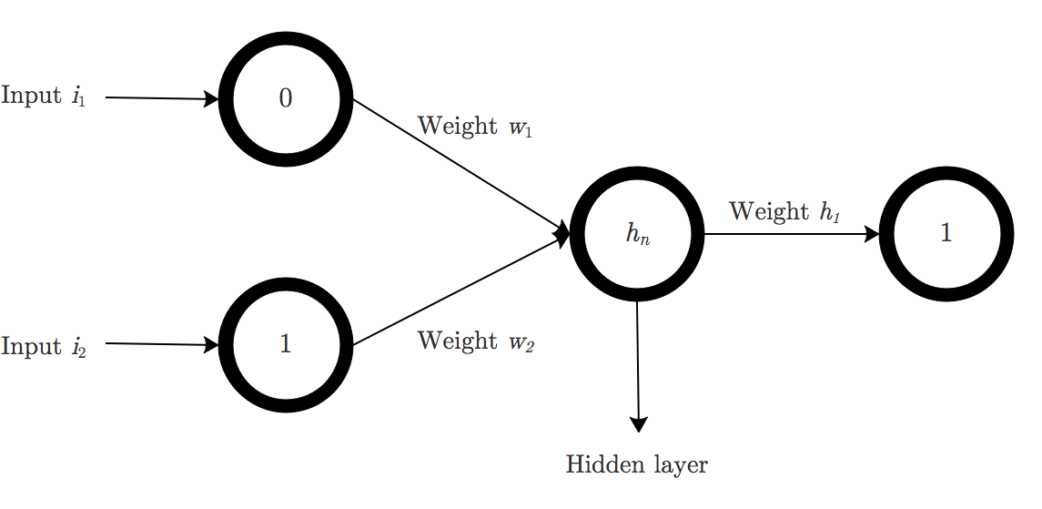
Here is a model of a neural network with one hidden layer:

It is overall very similar to the network we modeled above, but its learning capabilities will be slightly increased.

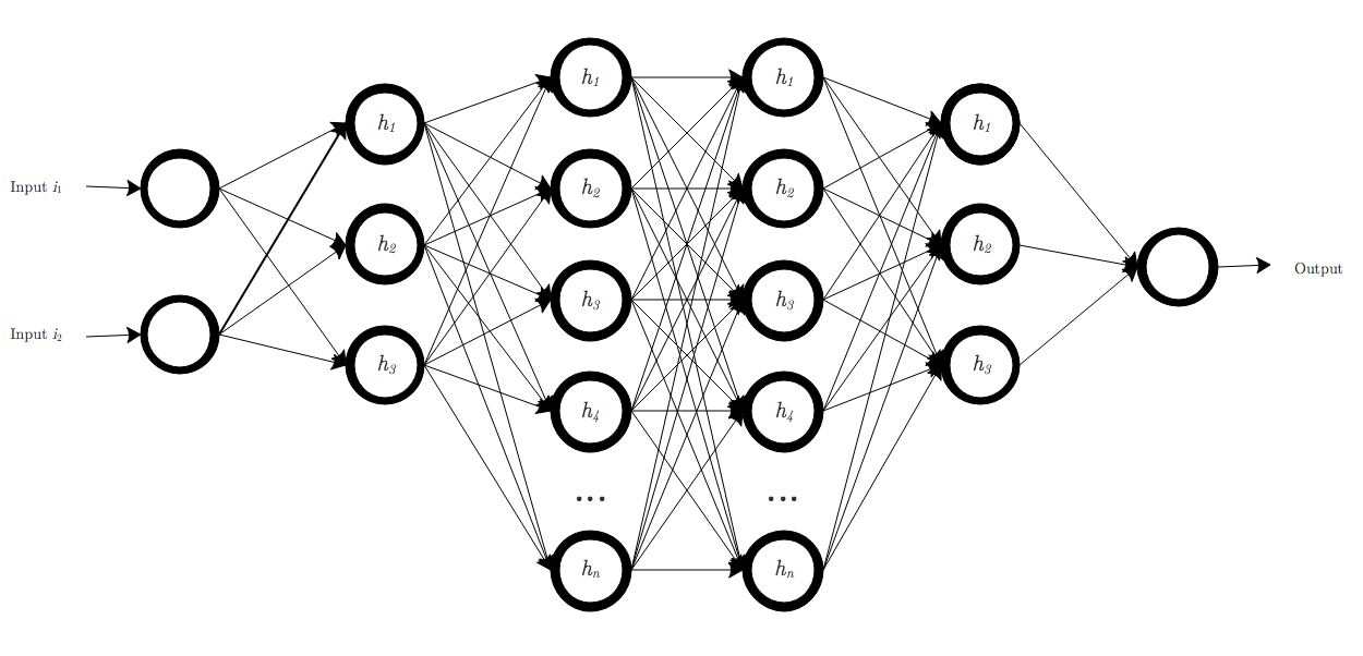
For comparison, here is a neural network with several more hidden layers:

These two examples are just vanilla feed-forward networks. There exists many types of neural network architectures, some of which are better suited than others for certain types of problems. This is also an open research field, with new kinds of architectures often leading to breakthroughs.

The limits of my sigmoid are the limits of my network

---

In the last post, we did a few calculations by hand to see what goes on under the hood when a neural network “learns”. However, the mathematically inclined reader may have noticed something wrong.

The XOR function simply cannot be learned by the one layer neural network. When a function is one-to-one, there is only one $x$ for every $y$. A one layer neural network can learn this type of function quite well, as it requires no complex calculations.

However, the XOR function is not one-to-one. There are two inputs for each output, both $[1, 0]$ and $[0, 1]$ output $1$, and both $[0, 0]$ and $[1, 1]$ output $0$. This is too nonlinear for the one layer network to learn.

Thus, the answer is to use a hidden layer. But more on this later.

But say we adjust the XOR function so that it is one-to-one:

Input 1	Input 2		Output
0	0		0
1	1		1
1	1		1
0	0		0

Even now, even though it is one-to-one, there issue in learning the trend still persists. Take a look at this example - upon plugging in the first input $0, 0$ into the equation $\sum_n i_n \cdot w_n$, using arbitrary weights of $.05$ and $.02$:

\[\sum_n i_n \cdot w_n = (0 \cdot 0.5) + (0 \cdot 0.2) = 0\]

then passing it through the sigmoid function:

\[\frac{1}{1 + e^{-(0)}} = 0.5\]

One ends up with an interesting answer of $0.5$. Now to pass this through the error-weighted derivative equation:

\[\text{ewd}(x) = \text{error} \cdot \text{input} \cdot \big(\text{output}\cdot (1 - \text{output})\big)\] \[\text{ewd}(x) = 0 \cdot 0 \cdot 0.5 \cdot (0.5) = 0\]

One ends up with 0, of course, because it needs no adjustment. However, because passing 0 through the sigmoid produces an output of $0.5$, the neural network will continously output $0.5$, when the correct answer is 0. As can be seen with our calculations, even with adjustments the output will not change.

One way around this is to change the activation function. Tanh, the sigmoid function’s close relative, is one we can look at briefly.

\[\text{tanh(x)} = \frac{-e^{-x}+e^x}{e^{-x}+e^x}\]

and its derivative:

\[\text{sech}^2\text{(x)} = \frac{2}{e^{-x}+e^x}\]

Here we are input our $\sum_n i_n \cdot w_n$ into the activation function tanh: \(\frac{-e^{-0}+e^{0}}{e^{-0}+e^{0}} = 0\)

Pass it through the derivative:

\[\frac{2}{e^{-(0)}+e^{0}} = 1\]

And finally through the error-weighted derivative equation:

\[\text{ewd(x)} = 0 \cdot 0 \cdot 1 = 0\]

As you can see, tanh is much better suited and will produce the correct output of 0. This demonstrates the large effect that the activation function can have on the quality of a neural network.

As mentioned in the last post, there are several other activation functions available for use, each with their own pros and cons. Some of the popular ones in use are tanh, ReLU, and Leaky ReLU.